SciPhysicsForums.com

[quote="FrediFizzx"] Here are the three hidden variables one of them of course being non-local.

1. The RandomChoice for A = lambda1
2. The RandomReal[] in the B line = lambda2
3. Sin[spin (β[[j]] - α[[j]])]^2 in the B line = lambda3
[/quote]
Correction: Number 1 is actually not a hidden variable. That is what QM predicts for A or B.

[quote="FrediFizzx"]So as I was saying, it is not possible to produce the negative cosine curve for EPR scenarios without some kind of hidden variable theory when using binary outcomes.[/quote]
Since quantum mechanics itself cannot produce the -cosine curve using binary outcomes for the EPR scenario, this seems to me to be a third strike against Bell's "theorem". A third strike means you are out. :)

IOW, Bell's model for local hidden variables is imposing something on those theories that QM can't even do since his model requires binary outcomes for A and B. So he was mixing apples and oranges basically. The other two strikes against Bell are;

1. It is mathematically impossible for anything to violate the inequalities.
2. [url=http://arxiv.org/abs/1103.1879]Joy Christian's local realistic model that gives the same prediction as QM for EPR-Bohm.[/url]

To date, Joy Christian's model is the only local realistic model that has perfect physical justification with a very simple physical postulate that is good common sense.

[quote="FrediFizzx"]Concerning the Mathematica code posted here that was furnished by [url=http://www.sciphysicsforums.com/spfbb1/viewtopic.php?f=6&t=192]John Reed[/url],

http://www.sciphysicsforums.com/spfbb1/download/Reed_Bell_EPR2.pdf

I have discovered that the so-called "quantum" section of that code is really not QM at all. It has three hidden variables and as we know there are no hidden variables in quantum mechanics. Here are the three hidden variables one of them of course being non-local.

1. The RandomChoice for A = lambda1
2. The RandomReal[] in the B line = lambda2
3. Sin[spin (β[[j]] - α[[j]])]^2 in the B line = lambda3

And it is pretty easy to realize just how un-physical those hidden variables are. So as I was saying, it is not possible to produce the negative cosine curve for EPR scenarios without some kind of hidden variable theory when using binary outcomes.[/quote]

You don't understand anything about this quantum mechanical simulation.

Concerning the Mathematica code posted here that was furnished by [url=http://www.sciphysicsforums.com/spfbb1/viewtopic.php?f=6&t=192]John Reed[/url],

http://www.sciphysicsforums.com/spfbb1/download/Reed_Bell_EPR2.pdf

I have discovered that the so-called "quantum" section of that code is really not QM at all. It has three hidden variables and as we know there are no hidden variables in quantum mechanics. Here are the three hidden variables one of them of course being non-local.

1. The RandomChoice for A = lambda1
2. The RandomReal[] in the B line = lambda2
3. Sin[spin (β[[j]] - α[[j]])]^2 in the B line = lambda3

And it is pretty easy to realize just how un-physical those hidden variables are. So as I was saying, it is not possible to produce the negative cosine curve for EPR scenarios without some kind of hidden variable theory when using binary outcomes.

Michel has kindly explained what is going on here. The polarization angle e for the particles is still there. It has just been set to a fixed angle of zero relative to a and b. I tried the above simulation with other fixed angles for e and it still works to produce the -cosine curve. It also works for spin 1 photons with e either fixed or random.

Recently on [url=http://challengingbell.blogspot.com/2015/06/a-flatlanders-view-on-joy-christians.html]Albert Jan's Blog[/url], we discovered that quantum theory cannot produce the negative cosine curve using +/-1 outcomes. So, how to best simulate what is going on in an EPR-Bohm scenario? It seems that one is forced to use some kind of hidden variable model to do it. Of course if anyone thinks they can do it without hidden variables, please post it here. :D

So I was playing around with John Reed's Mathematica version of Michel's epr-simple simulation and discovered that it can produce the -cosine curve without using the angle "e" for the particles. It now depends only on lambda, a and b. So the particles are only "carrying" lambda. Here are the links;

http://www.sciphysicsforums.com/spfbb1/EPRsims/EPRBsimJC_JR_MF.nb Mathematica notebook file.
http://www.sciphysicsforums.com/spfbb1/EPRsims/EPRBsimJC_JR_MF1.pdf PDF of notebook with results

[img]http://www.sciphysicsforums.com/spfbb1/EPRsims/EPRBsimJC_JR_MF.jpg[/img]

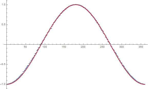
So this may be the most simple way to simulate EPR-Bohm giving the full -cosine curve using +/-1 outcomes for A and B with one degree resolution for the a and b angle difference. Of course Joy's S^3 simulations probably have the best [b]physics [/b]explanation.