I have simplified the code a bit so that I can understand what you are saying:
- Code: Select all
Angles = seq(from = 0, to = 360, by = 7.2) * 2 * pi/360
K = length(Angles) # The total number of angles between 0 and 2pi
corrs = matrix(nrow = K, ncol = K, data = 0) # Container for correlations
M = 10^4 # Size of the pre-ensemble. Next one can try 10^5, or even 10^6
r = runif(M, 0, 2*pi) # M uniformly distributed numbers between 0 and 2pi
z = runif(M, -1, +1) # M uniformly distributed numbers between -1 and +1
h = sqrt(1 - z^2)
x = h * cos(r)
y = h * sin(r)
e = rbind(x, y, z)
s = runif(M, 0, pi) # Initial states of the spins are the pairs (e, s) within S^3
f = -1 + (2/sqrt(1 + ((3 * s)/pi))) # For details see the paper arXiv:1405.2355
g = function(u,v,s){ifelse(abs(colSums(u*v)) > f, cos(Angles), 0)}
d = function(p,q){ifelse(2*acos(colSums(p*q)) < pi, 1, -1)}
for (i in 1:K) {
alpha = Angles[i]
a = c(cos(alpha), sin(alpha), 0) # Measurement direction 'a'
for (j in 1:K) {
beta = Angles[j]
b = c(cos(beta), sin(beta), 0) # Measurement direction 'b'
A = +sign(d(a,e)*g(a,e,s)) # Alice's measurement results A(a, e, s) = +/-1
B = -sign(d(b,e)*g(b,e,s)) # Bob's measurement results B(b, e, s) = -/+1
N = length((A*B)[A & B]) # Number of all possible events observed in S^3
corrs[i,j] = sum(A*B)/N # Product moment correlation coefficient E(a, b)
}
}
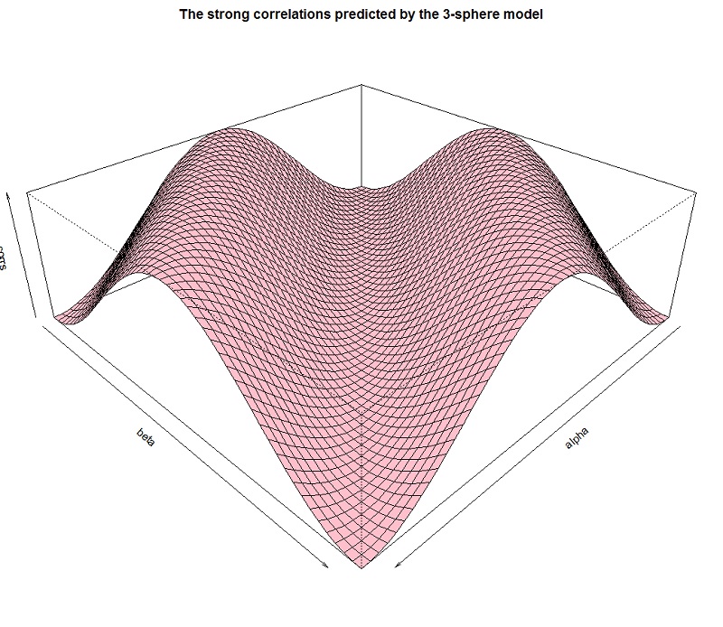
par(mar = c(0, 0, 2, 0))
persp(x = Angles, y = Angles, main = "The strong correlations predicted by the 3-sphere model", z = corrs, zlim = c(-1, 1), col = "pink", theta = 135, phi = 30, scale = FALSE, xlab = "alpha", ylab = "beta")
***